A blog posts by Derik Verkest and Bo Nash
Experiment Summary
In order to understand the context of this experiment it is important to learn some key terms first. As mentioned in the title of this blog post, pheonology is what this experiment was about. “Phenology is the study of the timing of cyclical events in an organism’s life cycle, such as the flowering plants, emergence of worker bees from the hive, or the migration of birds.” (lab manual)
The phenology of organisms is pushed into action or “cued” by environmental factors such as seasonal temperature change, photoperiod (daylight), or precipitation (i.e. rain, snow, etc.). This is why climate change presents such a drastic problem for global ecosystems and organisms, it not only changes the climate but also shifts the behaviors and important life functions of many living things. The experiment that was conducted had several goals/objectives.
- Define phenology
- Discuss examples of phenological events
- Distinguish between continuous and categorical data
- Create a scatterplot and a bar graph
- Identify trends in long-term climate data
- Describe correlations between climate data and phenology
- Predict the effects of phenology shifts on interspecific interactions
Data
Throughout the experiment that was conducted, data sets were used to analyze changes in temperature and organism behavior. Data comes in many helpful forms and in this experiment in particular the use of graphs shows a great visual representation of numerical data that would otherwise be hard to understand. For the sake of simplicity and organization we will define data into two categories: continuous and categorical. Continuous data is more well-known as quantitative data and are variables that can be measured on a numerical scale. Categorical data is more well-known as qualitative data and can be divided into distinct groups determined by qualitative properties. Examples of continuous data are height, weight, temperature, and salinity. Categorical data can be seen as sex, age group (years), hair color, and seasons. Finding and presenting data doesn’t accomplish much if there is not way to see the “center” or “spread” of the data. The most common way of measuring this is called the mean, which averages all the possible values in a given data set.
Visual Representation (Graphs)
Graphs are a neat and common way of presenting numerical data visually to the intended audience. Most, if not all, graphs that ecologists create uses the mean that was previously talked about in the last paragraph. There are two mathematical ways that scientists can indicate how close or far away data is from the mean: standard deviation and standard error. standard deviation “indicates how widely scattered individual scores are” while standard error “…a measure of uncertainty around the mean measurement.” (lab manual). The majority of the graphs present will be scatter plots and bar graphs. This experiment will be divided into “Activity 1” and “Activity 2”. These activities will use all of the previously mentioned information in order to see trends in temperature and how that correlates to organisms’ phenology.
Activity 1: Long-term temperature trends
–Long-Term Temperature Trends–
The mean temperatures being shown in the graphs below were collected as monthly mean temperatures by the United Kingdom Meteorological Office from 1659-2016 in the cities of London, Bristol, and Preston.
The variable plotted on the x-axis is the year the data was collected, and on the y-axis is the mean temperature that was recorded for that year. This was done in order to clearly show the trend when comparing temperature to the year associated with it, because if they swapped positions then it would be difficult to see the linear progression associated with such trend.
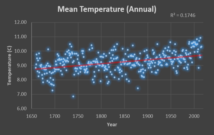
Based on the trend lines for the mean annual temperatures, mean Feb-Apr temperatures, and mean Mar-May temperatures, it appears that the mean temperatures for the last three hundred and seventy years has uniformly increased at a reasonably constant rate. This rate has been roughly one degree every three hundred years. The correlation coefficient (R2) represents how strong the relationship is between two variables. This relationship has a scale range of 0-1. The closer R2 is to 1, the stronger the relationship between the two variables. The graphs above all show their R2 in the top right corners. When comparing R2 between Feb-Apr mean temperatures and the Mar-May mean temperatures, we see that the Mar-May temperatures have the greater R2 value of 0.101. This implies that the data recorded forms a more related connection; hence a more correlated trend line is being shown.
Activity 2: Pollination of the Early Spider Orchid (Ophrys sphegodes) by the Solitary Bee (Andrena nigroaenea)
Like most symbiotic relationships between animals and plants, this one in particular involves the Solitary Bee pollinating the Early Spider Orchid. One of the main types of phenology is the flowering of plants and in this instance scientists gathered data from 77 species of the early spider Orchid during the time span of 1848-1958. Using this data along with field observations of Spider Orchids in a single population in the UK between 1975 and 2006, the scientists were able to determine the peak flowering dates for each year. By analyzing this graph you can see how there was been a trend in the fact that the peak flowering time at the end of the century has moved sooner to March 1 by around 3 days compared to the beginning of the century.
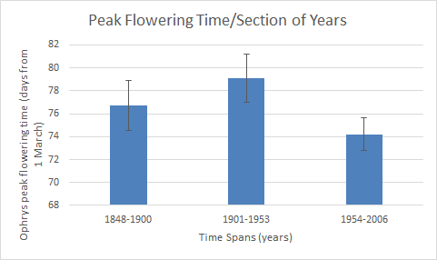
Credit: Bo Nash
In order to see if there was a correlation between the first flight of the Solitary Bees and the flowering time, scientists and citizen scientist between 1975 and 2009. Researchers also examined specimens of Solitary Bees in the Natural History Museum in London in order to obtain a more comprehensive look at the data. The bar graph below shows the correlation between first flight and time span of years. The bar below also shows that in the last period of years it is shown that bees are having their first flight earlier than at the beginning of the last century.
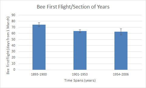
Credit: Bo Nash
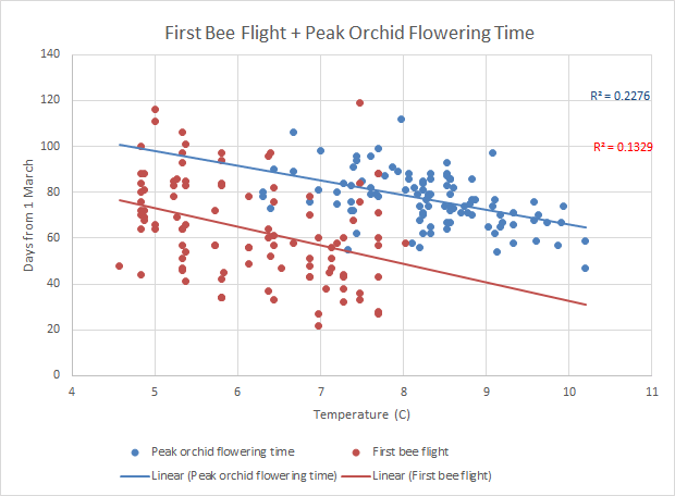
Although these two bar graphs are useful at showing individual data, the combined data is what we’re interested in. In the scatter plot below there is combined data points of peak orchid flowering time (blue) and first bee flight (red) vs. the mean spring temperature. At 7C the bees are first have their first flight before the peak flowering time. Compared to 10C when the Bees weren’t measured to have a first flight but the orchids were at peak flowering.
Credit: Bo Nash
After analyzing all of this information and looking at the graphs I can predict that if the global temperature continues to increase, the Early spider Orchid might miss out on the Solitary Bee’s first flight, seeing from the previous chart that there is not bee flight over about 8C.
Brood Awakening
After completing this lab and analyzing how phenology of organisms it has become easier to analyze current ecological situations and determine if there is a change in phenology involved. One such example has to do with the cicada outbreak and the earlier-than-usual presence of cicadas. Cicadas arrived in the North and Midwest of the United States in 2017 almost 4 years earlier than usual (Sheik). After analyzing the information in the research article and comparing it to our lab, there was a correlation. The increase in annual temperature caused the bees to have their first-flight significantly earlier. This was almost the exact same scenario as what happened with the cicadas. The increase in global average temperature caused the nymph cycle of cicadas to be altered, thus making them arrive four years earlier. Although this was an obvious pattern that could be depicted, another hypothesis to explain the cicada emergence in 2017 is that the internal clock in their brains could have been skewed by some environmental factor during reproduction.
Climate Change In Everyday Life
Climate change is considered the global problem of this generation. The possibility of a changed global environment and what that can induce is daunting and quickly approaching. The effects of climate change are already affecting the general public today. The fires in Australia are being attributed to a drought that is the result of the changing climate. The fire season is longer and precipitation is lower. (USA Today). The smoke from the fires is being carried into major cities and is causing the breathing air to become unsafe. Although this along with the increasing amount of heat waves per year are considered obvious effects of climate change, communicating it to the public is difficult. Americans are almost evenly split on climate related issues. 48% believe that climate change is due to human activity (Pew). This shows that the main challenge to communicate the general public about climate change is the current state of the public. People are more skeptical than ever and a lot ignore scientific data even thought that is considered fact. In order to communicate the fact that climate change is real we as science communicators need to show that there is a direct correlation between the heatwaves, the fires, and the floods that everyday people are experiencing is caused by climate change. The effects of climate change are far reaching and even effect the basic necessity for all life: water. This is shown in the following publication:
Peer Review Citation: Baba, A., & Baba, A. (2011). Climate Change and its Effects on Water Resources: Issues of National and Global Security. Place of publication not identified: Springer.
Credits
Bo Nash: “Experiment Summary”, “Activity 2” information and graphs, “Climate Change in Everyday Life”
Derik Verkest: “Activity 1” information and graphs, “Brood Awakening”
Works Cited
- “Americans’ Views on Climate Change and Climate Scientists.” Pew Research Center Science & Society, Pew Research Center, 30 Dec.2019, http://www.pewresearch.org/science/2016/10/04/public-views-on-climate-change-and-climate-scientists/.
- Robbirt et al., 2014. Pollination of the early Spider Orchid (Ophrys sphegodes) by the Solitary Bee.
- Sheikh, Knvul. “Brood Awakening: 17-Year Cicadas Emerge 4 Years Early.” Scientific American, Scientific American, 26 May 2017, http://www.scientificamerican.com/article/brood-awakening-17-year-cicadas-emerge-4-years-early/.
- Siren, A., Nowak, J., Bryan, A., Ivan, J., Zimova, M., Sirén, A., … Morellato, P. (2019). Local climate determines vulnerability to camouflage mismatch in snowshoe hares. Global Ecology & Biogeography. https://doi.org/10.1111/geb.13049

